Dice Recognition — Phase 2

D20 dice models sourced from this set on CGTrader.
Optimised from 25MB to 149KB for WebGL scene above.

Overview

Phase 1 proved the concept. Synthetic data generated inside a game engine, zero real world images, 90% mAP50 on a first pass. That was the good news.

The bad news was visible the moment real world inference started — jumpy predictions, missed detections on certain faces, and a model that had clearly never seen a real camera, real lighting or a real die before. The confusion matrix told the story plainly. D6_2 and D6_3 were confusing each other constantly. D6_3 had a background miss rate of 228 — meaning the model simply failed to detect the die at all on that face more often than felt acceptable.

Three things needed fixing:

• The sim-to-real gap — the model had never seen a real die
• The inference tool — single frame predictions were too noisy to be useful
• The training run — the loss curves showed the model hadn't finished learning at epoch 50

Phase 2 tackles all three.

Closing the Sim-to-Real Gap

The sim-to-real gap is the performance drop that happens when a model trained entirely on synthetic data meets the real world for the first time. Synthetic renders are clean, perfectly lit and geometrically precise. Real cameras have lens distortion, compression artefacts, inconsistent lighting and surfaces that don't behave like Unity materials.

The fix isn't to abandon synthetic data — it's to add a small amount of real world data alongside it. Even a modest number of real images gives the model a bridge between the two worlds.

Capturing Real World Images

This was the painful bit I was trying to avoid, but as mentioned purely synthetic data can have issues when the model sees the real world and we have to be thankful that it wasn't manually taking 6000 plus images of each face and manually annotating them.

I built a simple webcam capture tool in Python — space bar to capture, counter overlay on screen, images saved with timestamps.

The process was straightforward but deliberate. For each face value I placed the die in front of the webcam and captured around 50 images, moving it slightly between each shot — different position in frame, slight rotation, occasionally closer or further from the camera. Different lighting conditions where possible. The goal was variety, not perfection.

336 images in total across all six face values. Around 56 per class.

Annotating with Roboflow

Hindsight showed me this was actually the most laborious part of the process and gave me a clear marker for some improvements later down the line (shameless foreshadowing!)

Unlike the synthetic pipeline where annotations are written automatically, real world images need manual bounding boxes. I used Roboflow's annotation tool for this — draw a box around the die, assign the class label, move to the next image.

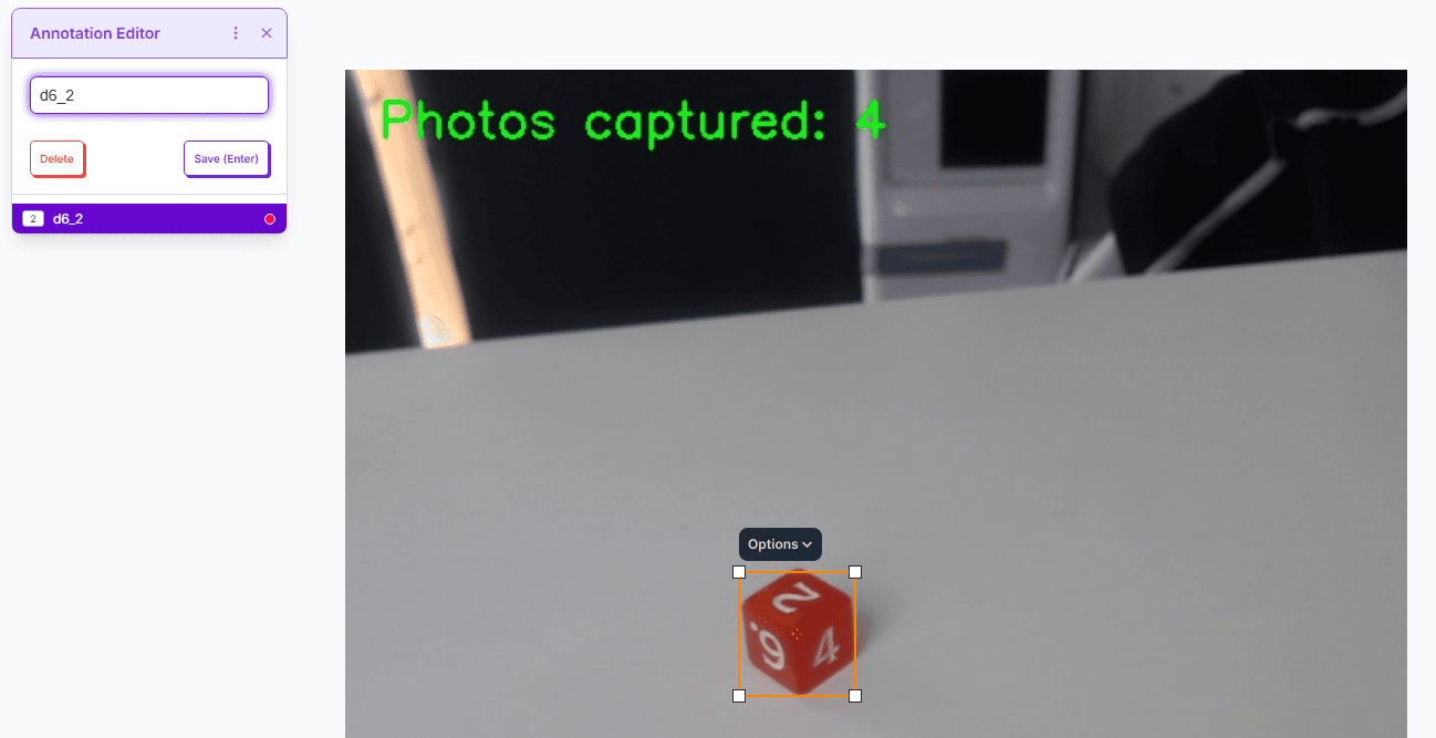
A couple of things worth noting from the annotation process. The class indices needed careful verification — d6_1 must be class 0, d6_2 class 1, and so on, matching the synthetic data exactly. A mismatch here would silently corrupt the training signal. I spot checked images against their label files to confirm everything lined up.

The annotation style was kept consistent with the synthetic data — whole die bounding box, not tight to individual faces. Consistency between real and synthetic annotations matters more than perfect precision on either.

Mixing the Datasets

With annotations exported from Roboflow in YOLOv8 format, the merge was simple — images and label files copied into a new folder alongside the 3,000 synthetic ones.

336 real images alongside 3,000 synthetic. Roughly 10% of the total dataset. That ratio felt right — enough to matter, not so much that the synthetic variety gets diluted.

Second Training Run (v2)

With the expanded dataset ready — 3,336 images, real and synthetic mixed — it was time to train properly.

The v1 results.png had shown loss curves still declining at epoch 50. The model wasn't done. So v2 ran for 100 epochs instead of 50, giving it the time it was clearly asking for.

Configuration

• Model: YOLOv8n — same architecture, pretrained COCO weights
• Dataset: 3,336 images (3,000 synthetic + 336 real)
• Epochs: 100 | Batch size: 16 | Device: GTX 1060

Training took approximately 6–7 hours on the GTX 1060.

v2 Results

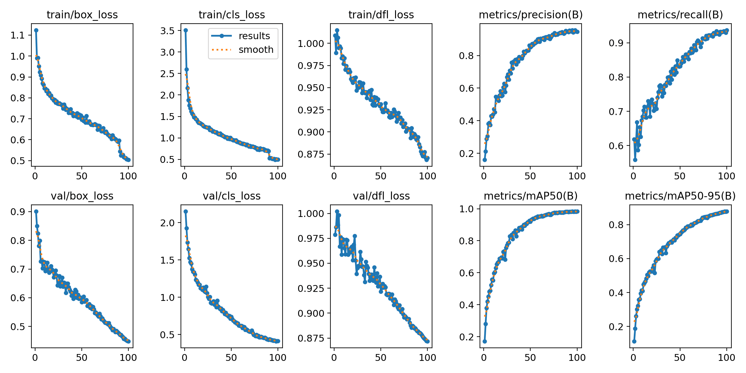
The numbers were a significant step forward:

Metric	v1	v2
mAP50	~0.90	0.9828
mAP50-95	~0.75	0.8718
Precision	~0.85	0.9373
Recall	~0.85	0.9822
cls_loss	0.7737	0.4969

The classification loss dropped 36% — the model became significantly more confident about which face value it was seeing. Recall hitting 98.2% meant it was now finding the die in almost every frame. And crucially, the loss curves at epoch 100 were much flatter than at epoch 50 in v1. The model had actually converged this time.

The outsized impact of the real world photos is worth pausing on. 336 images — about 10% of the dataset — produced a 9 percentage point improvement in mAP50. Small amounts of real data have disproportionate impact on a synthetically trained model. That's the key finding from Phase 2.

Fixing the Inference Tool

The v1 inference was a single predict call — one frame, one prediction, display it on screen. Functional but noisy. Watching it in real use the class label flickered constantly even with the die sitting completely still.

The fix was temporal aggregation — rather than trusting any single frame, collect predictions across a rolling window and only confirm a result when enough frames agree.

So this time it was a python script again which opened the webcam, keeping high confidence frames over time and keeping them to determine the overall confidence threshold and report it on the webcam itself. Went with the following settings...

STABILITY_FRAMES = 15
AGREEMENT_THRESHOLD = 0.7  # 70% of frames must agree

# Only confirm when threshold is met
if most_common_count / STABILITY_FRAMES >= AGREEMENT_THRESHOLD:
    confirmed_result = predicted_value

The difference in practice was immediate. Instead of flickering between d6_5 and d6_6 every other frame, the tool now waits until it has seen enough consistent evidence before committing to a result. A stability counter shows how the buffer is filling. Once confirmed, the result stays on screen until reset.

As you can see from the video, the detection had greatly improved when using the same die to test, but if you are like me, at this point I was thinking "Hold on, what if I had just made the model better at spotting that die and not improved inference overall."

Well luckily I had my sons dice I could test with...

Testing on a Different Die

The real test of any model trained on specific data is whether it works on data it has never seen. My son's d6 is noticeably different from mine — darker colour, different font weight, different plastic finish. It wasn't in the training data at all.

First pass results with the v2 model on his die: approximately 70% accuracy.

That number sounds underwhelming until you consider what it actually means. The model was trained entirely on one specific die (and a handful of synthetic variants). It had never seen his die. 70% on first contact with completely unseen dice is genuine generalisation, not memorisation.

The remaining failures were mostly on faces 5 and 6 — the most visually similar pair in the confusion matrix — and the occasional missed detection at shallow camera angles. Consistent with what the confusion matrix predicted.

What the Numbers Actually Mean

mAP50 of 0.9828 is a good number but it can feel abstract. In practical terms for this use case:

Precision at 93.7% means when the model says "that's a d6_4" it's right 19 times out of 20. Recall at 98.2% means it finds the die in 98 frames out of every 100. Combined with temporal aggregation — which requires 70% agreement across 15 frames before confirming — the system reliability in practice is higher than either individual metric suggests.

A single frame accuracy of 95% across 15 frames means the probability of getting a wrong confirmed result is extremely low. The occasional bad frame gets outvoted.

100% accuracy isn't the goal and isn't achievable. The goal is reliable detection within a defined operating envelope — reasonable lighting, camera at 30 degrees or more above horizontal, die clearly visible. Within that envelope the v2 model is genuinely production-ready for the next stage.

What the Confusion Matrix Now Shows

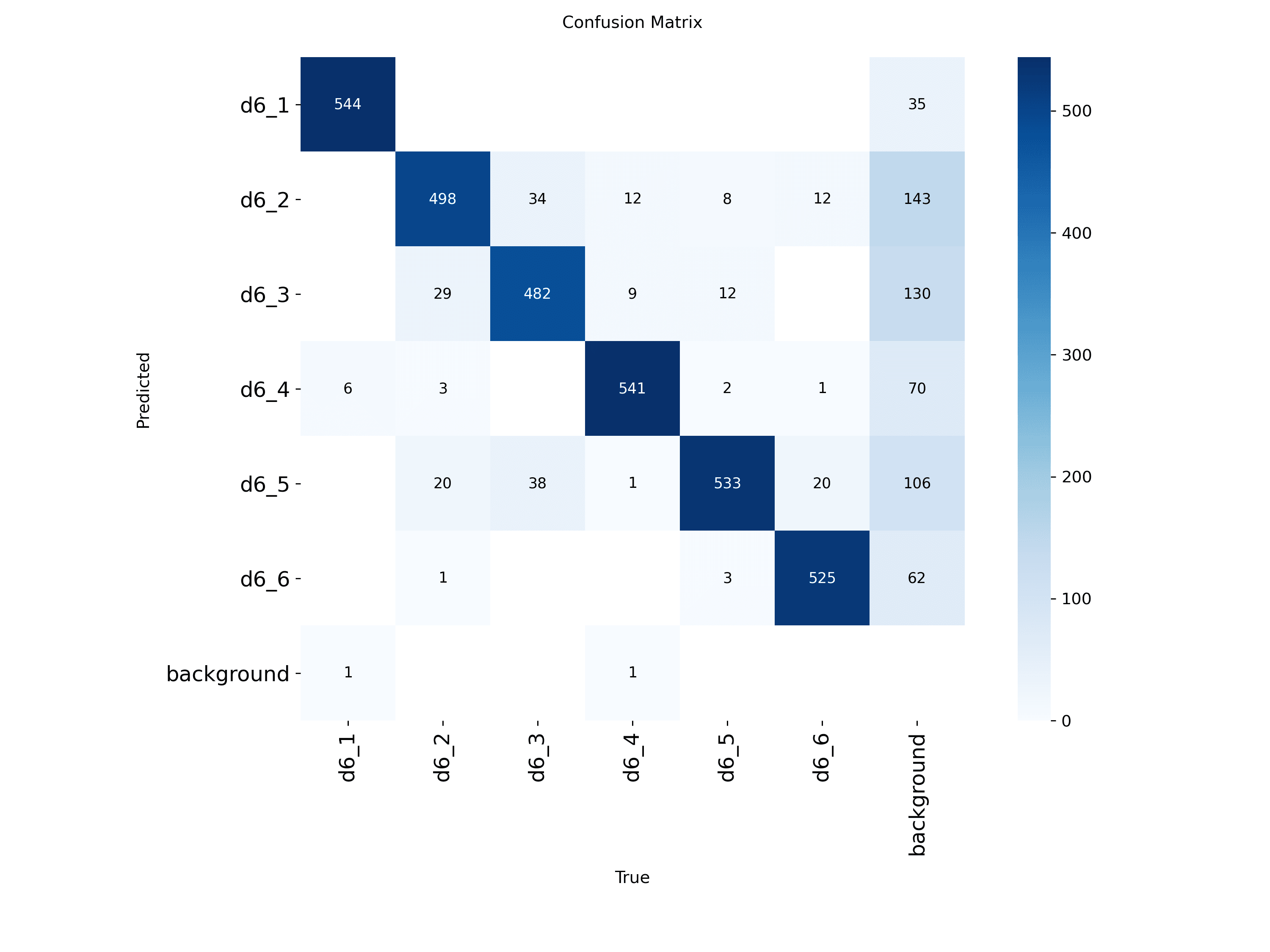
The diagonal is much darker and the off-diagonal noise is much reduced compared to v1. The background column — missed detections — is notably smaller across all classes. D6_2 and D6_3 still show some mutual confusion but it's substantially improved. D6_1 and D6_4 are essentially clean.

Next Steps

Phase 2 has a working, validated model with genuine real world generalisation. Phase 3 is about making the detection smarter.

The main items on the roadmap:

• Top face annotation — rather than annotating the whole die, annotate only the top face using Unity's knowledge of the die's exact 3D orientation. This directly teaches the model which face is "up" rather than relying on it figuring that out implicitly from viewing angle.
• More synthetic data — 6,000 images instead of 3,000, with tighter elevation control

If you made it this far, then thank you for putting the time in to read the article.